1. Introduction
This report will be submitted as a peer review assignment at the end of the third week of the Data Science as a Field Course. The NYPD Shooting Incident Data is downloaded from the City of New York website. The data set contains records of shooting incidents that happened between 2006 and 2021. I will do an analysis of the area, age group, sex and race.
2. Data Wrangling
2.1 Loading Libraries
library(tidyverse)
library(lubridate)
library(prettydoc)
library(xtable)
library(knitr)
2.2 Data Import
I am importing the csv file that I downloaded and placed inside the data directory. The link to the data set is https://data.cityofnewyork.us/Public-Safety/NYPD-Shooting-Incident-Data-Historic-/833y-fsy8. The webpage also provide information for the different columns.
shooting_data <- read_csv("data/NYPD_Shooting_Incident_Data__Historic_.csv")The dataset contains 25596 Rows and 19 Columns.
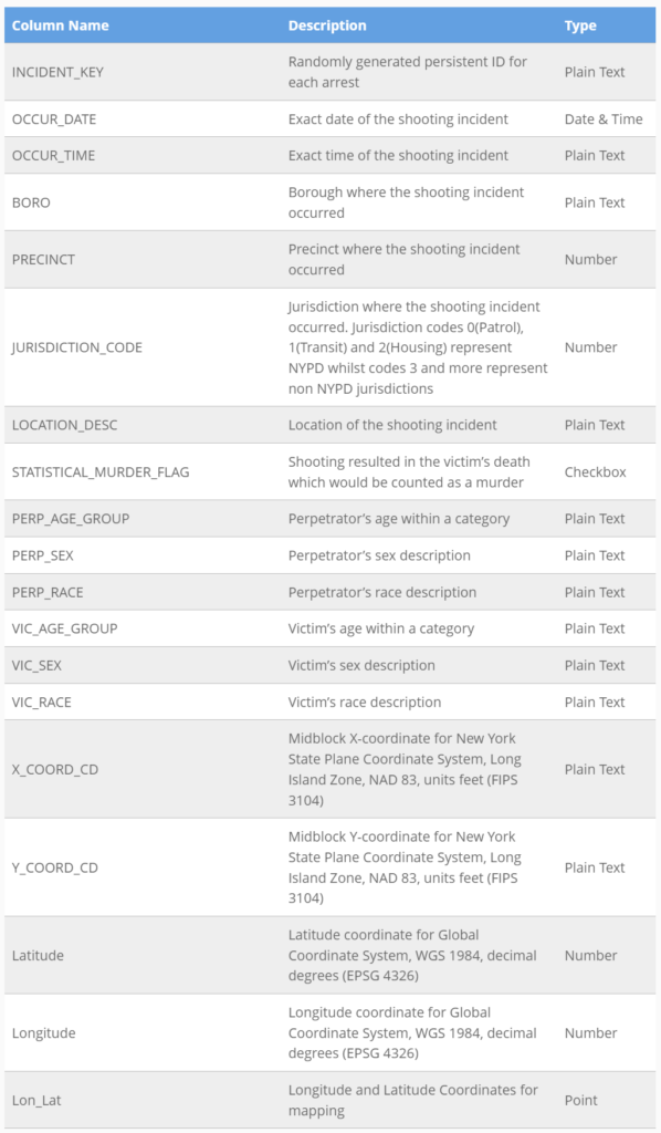
The column name, Description and Data Type of each Columns as indicated on the City of New York website is listed below in table format.
2.3 Tidy Data
I will not be doing any spatial analysis and therefore I won’t need the spatial fields. I will also remove the Incident Key, Precinct and Jurisdiction.
shooting_data <- shooting_data %>%
  select(-INCIDENT_KEY, -PRECINCT, -JURISDICTION_CODE,
         -X_COORD_CD, -Y_COORD_CD, -Latitude, -Longitude, -Lon_Lat)
After looking at the first 10 rows, we can see that the data is in a tidy format. I used the lubridate package to change the OCCUR_DATE field to a date object and the OCCUR_TIME field to a time object. I also changed all categorical data to factors and changed the STATISTICAL_MURDER_FLAG from True and False to Yes and No.
When looking at the summary of the data, we can see that the fields related to the Perpetrator contains a lot of missing values. My assumption is that these are cases where the perpetrator has not been apprehended yet. I might want to see the ratio of closed cases to total cases, and therefore I will not remove these missing values. The LOCATION_DESC field also contain a lot of missing values and I decided to remove that column as a whole.
head(shooting_data)

shooting_data <- shooting_data %>%
  mutate(OCCUR_DATE = mdy(OCCUR_DATE),
         OCCUR_TIME = hms(OCCUR_TIME))

shooting_data$BORO <- as.factor(shooting_data$BORO)

shooting_data$STATISTICAL_MURDER_FLAG <- as.factor(shooting_data$STATISTICAL_MURDER_FLAG)
levels(shooting_data$STATISTICAL_MURDER_FLAG)[1] <- "No"
levels(shooting_data$STATISTICAL_MURDER_FLAG)[2] <- "Yes"
shooting_data$STATISTICAL_MURDER_FLAG <- factor(shooting_data$STATISTICAL_MURDER_FLAG, levels = c("Yes", "No"))

shooting_data$PERP_AGE_GROUP <- as.factor(shooting_data$PERP_AGE_GROUP)
shooting_data$PERP_SEX <- as.factor(shooting_data$PERP_SEX)
shooting_data$PERP_RACE <- as.factor(shooting_data$PERP_RACE)
shooting_data$VIC_AGE_GROUP <- as.factor(shooting_data$VIC_AGE_GROUP)
shooting_data$VIC_SEX <- as.factor(shooting_data$VIC_SEX)
shooting_data$VIC_RACE <- as.factor(shooting_data$VIC_RACE)

head(shooting_data)

summary(shooting_data)

shooting_data <- shooting_data %>%
  select(-LOCATION_DESC)
3 Data Exploration
3.1 Transformation
I would like to see the number of shootings per year as well as the percentage of the total. I start by adding a field for the year, grouping by year and calculating the percentages.
shooting_data_per_year <- shooting_data %>%
  mutate(year = format(as.Date(OCCUR_DATE), format = "%Y")) %>%
  group_by(year) %>%
  count() %>%
  mutate(per_year = round((n/nrow(shooting_data)*100),2))

kable(shooting_data_per_year,
      col.names = c("Year",
                    "Number of Shootings",
                    "Percentage"))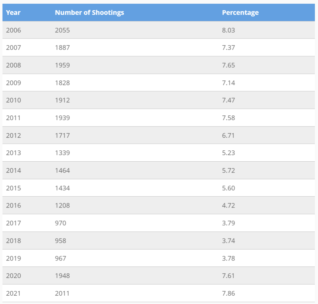
I would also like to see the percentages for the other categorical data.
shooting_data_boro <- shooting_data %>%
  group_by(BORO) %>%
  count() %>%
  mutate(per_boro = round((n/nrow(shooting_data)*100),2))%>%
  arrange(n)

kable(shooting_data_boro,
      col.names = c("Borough",
                    "Number of Shootings",
                    "Percentage"))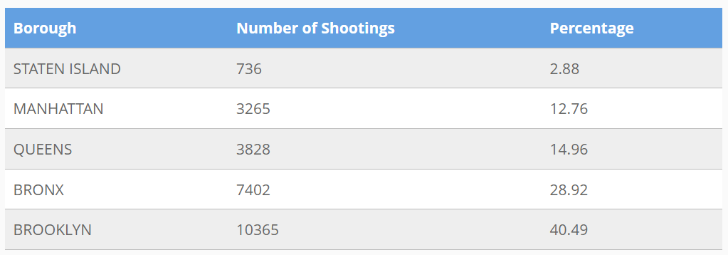
shooting_data_murder <- shooting_data %>%
  group_by(STATISTICAL_MURDER_FLAG) %>%
  count() %>%
  mutate(per_murder = round((n/nrow(shooting_data)*100),2))

kable(shooting_data_murder,
      col.names = c("Murder",
                    "Number of Shootings",
                    "Percentage"))
There are three levels with only one value in them that I excluded from the perpetrator age table. The levels are “1020”, “224” and “940”. I also excluded the unknown level.
shooting_data_perp_age_group <- shooting_data %>%
  filter(PERP_AGE_GROUP != "1020" & PERP_AGE_GROUP != "224" & PERP_AGE_GROUP != "940" & PERP_AGE_GROUP != "UNKNOWN")

shooting_data_perp_age_group_total <- nrow(shooting_data_perp_age_group)

shooting_data_perp_age_group <- shooting_data_perp_age_group %>%
  group_by(PERP_AGE_GROUP) %>%
  count() %>%
  mutate(per_perp_age_group = round((n/shooting_data_perp_age_group_total) * 100,2))

kable(shooting_data_perp_age_group,
             col.names = c("Age Group",
                           "Number of Shootings",
                           "Percentage"))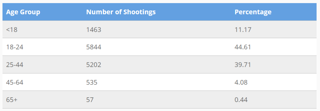
I removed the Unknown and NA levels from the perpetrator sex table.
shooting_data_perp_sex <- shooting_data %>%
  filter(PERP_SEX != "U" & PERP_SEX != "NA")

shooting_data_perp_sex_total <- nrow(shooting_data_perp_sex)

shooting_data_perp_sex <- shooting_data_perp_sex %>%
  group_by(PERP_SEX) %>%
  count() %>%
  mutate(per_perp_sex = round((n/shooting_data_perp_sex_total) * 100,2))

kable(shooting_data_perp_sex,
             col.names = c("Sex",
                           "Number of Shootings",
                           "Percentage"))
I removed the Unknown level from the perpetrator race table.
shooting_data_perp_race <- shooting_data %>%
  filter(PERP_RACE != "UNKNOWN")

shooting_data_perp_race_total <- nrow(shooting_data_perp_race)

shooting_data_perp_race <- shooting_data_perp_race %>%
  group_by(PERP_RACE) %>%
  count() %>%
  mutate(per_perp_race = round((n/shooting_data_perp_race_total) * 100,2)) %>%
  arrange(n)

kable(shooting_data_perp_race,
             col.names = c("Race",
                           "Number of Shootings",
                           "Percentage"))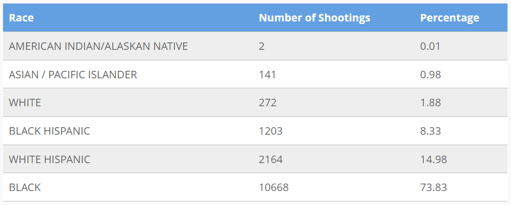
shooting_data_vic_age_group <- shooting_data %>%
  group_by(VIC_AGE_GROUP) %>%
  count() %>%
  mutate(per_vic_age_group = round((n/nrow(shooting_data) * 100),2))

kable(shooting_data_vic_age_group,
             col.names = c("Age Group",
                           "Number of Shootings",
                           "Percentage"))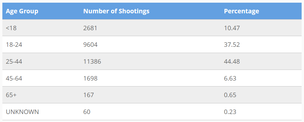
shooting_data_vic_sex <- shooting_data %>%
  group_by(VIC_SEX) %>%
  count() %>%
  mutate(per_vic_sex = round((n/nrow(shooting_data) * 100),2))

kable(shooting_data_vic_sex,
             col.names = c("Sex",
                           "Number of Shootings",
                           "Percentage"))
shooting_data_vic_race <- shooting_data %>%
  group_by(VIC_RACE) %>%
  count() %>%
  mutate(per_vic_race = round((n/nrow(shooting_data) * 100),2)) %>%
  arrange(n)

kable(shooting_data_vic_race,
             col.names = c("Race",
                           "Number of Shootings",
                           "Percentage"))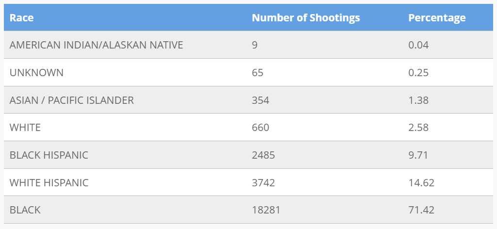
3.2 Visualisation
I will start of by creating bar graphs for all of the categorical data. This will help to get a better understanding of the data and might lead to more questions.
The first plot shows the number of shootings per year. We can see a decline from 2012 to 2019 and then a huge increase between 2020/21.
year_plot <- ggplot(data=shooting_data_per_year, aes(x=year, y=n)) +
  geom_bar(stat='identity', color = "#339FFF", fill = "#339FFF") +
  ggtitle("Total Shootings per Year") + xlab("Year") + ylab("Number of Shootings")

year_plot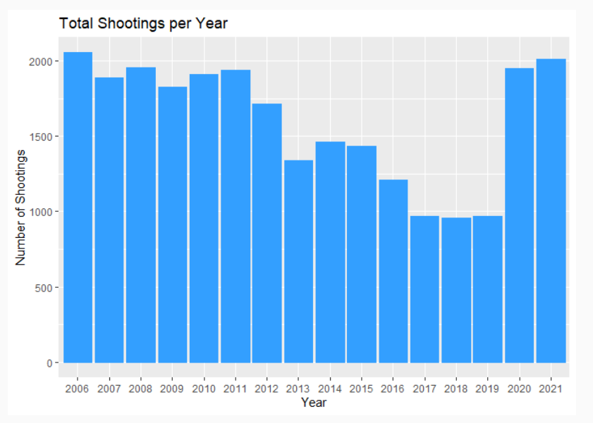
The next graph show the number of shootings per Borough for the complete data set (2006 – 2021). BROOKLYN has the most shootings at a Total of 10365 shootings and STATEN ISLAND the least with 736 shootings. I am not familiar with the occupancy of these Boroughs and will need some further research to understand if the numbers are related to occupancy.
boro_plot <- ggplot(data=shooting_data_boro, aes(x=reorder(BORO,(n)), y=n)) +
  geom_bar(stat='identity', color = "#339FFF", fill = "#339FFF") +
  ggtitle("Total Shootings per Borough") + xlab("Borough") + ylab("Number of Shootings")

boro_plot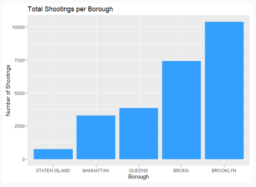
When the victim died as a result of the shooting it is classified as a murder. There are 4928 Deaths which translates to 4928 Murders. The remaining 20668 victims survived the shooting.
murder_plot <- ggplot(data=shooting_data_murder, aes(x=reorder(STATISTICAL_MURDER_FLAG,(n)), y=n)) +
  geom_bar(stat='identity', color = "#339FFF", fill = "#339FFF") +
  ggtitle("Murder Classifications") + xlab("Death") + ylab("Total")

murder_plot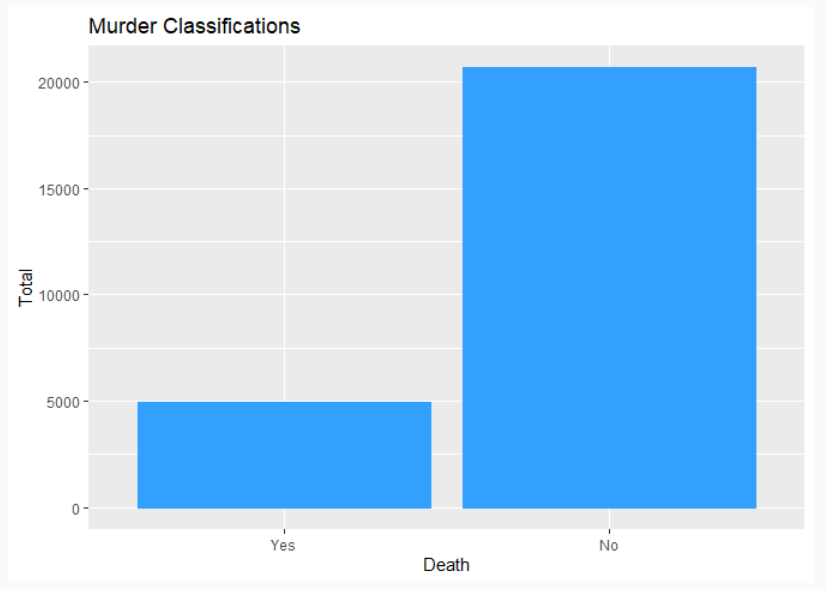
I created a bar plot to determine the Age Groups of most perpetrators. From the graph it can be seen that the majority of perpetrators are between 18 and 24 years old.
perp_age_group_plot <- ggplot(data=shooting_data_perp_age_group, aes(x=PERP_AGE_GROUP, y=n)) +
  geom_bar(stat='identity', color = "#339FFF", fill = "#339FFF") +
  ggtitle("Perpetrator Age Group") + xlab("Age Group") + ylab("Total")

perp_age_group_plot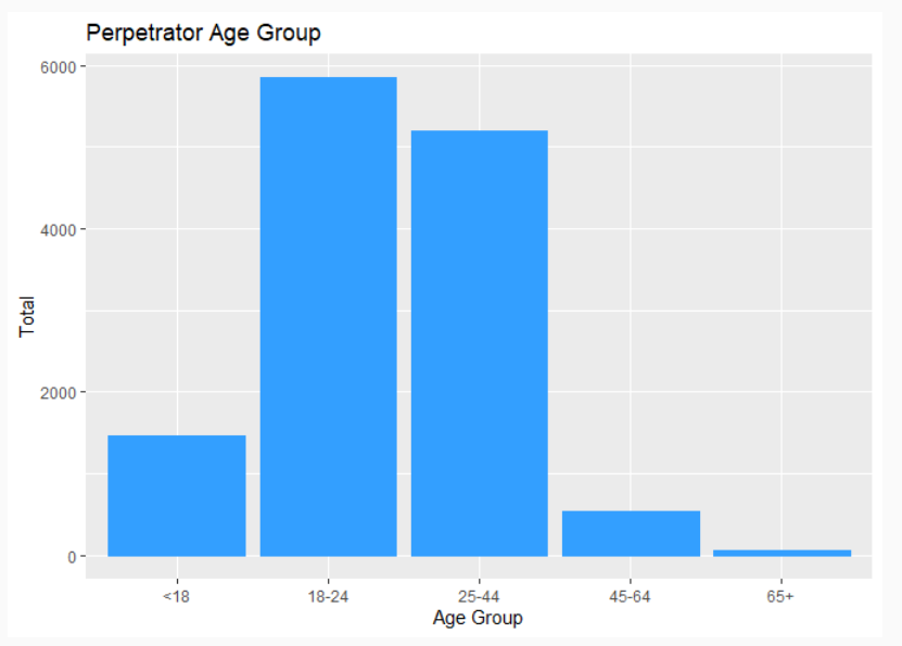
The sex of perpetrators was another category that I wanted to analyse. When looking at the bar graph it is evident that the majority of perpetrators are Male, the are very few Female perpetrators.
perp_sex_plot <- ggplot(data=shooting_data_perp_sex, aes(x=PERP_SEX, y=n)) +
  geom_bar(stat='identity', color = "#339FFF", fill = "#339FFF") +
  ggtitle("Perpetrator Sex") + xlab("Sex") + ylab("Total")

perp_sex_plot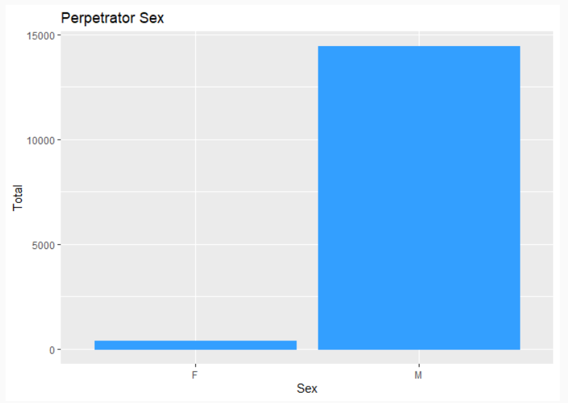
The last category of perpetrators that I wanted to look at, was race. We can see that most perpetrators are black. However, without knowing the overall population distribution it is difficult to draw any conclusions. It might be possible that the majority of the population is black people.
perp_race_plot <- ggplot(data=shooting_data_perp_race, aes(x=reorder(PERP_RACE,(n)), y=n, color = PERP_RACE, fill = PERP_RACE)) +
  geom_bar(stat='identity') +
  theme(axis.text.x=element_blank(), axis.ticks.x=element_blank()) +
  ggtitle("Perpetrator Race") + xlab("Race") + ylab("Total")

perp_race_plot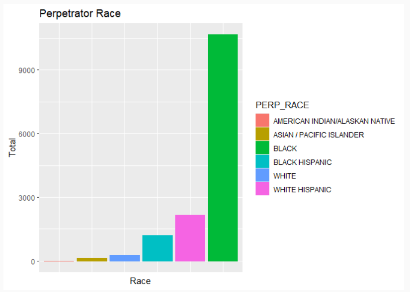
When looking at the Age Groups of most victims it can be seen that the majority of victims are between 25 and 44 years old.
vic_age_group_plot <- ggplot(data=shooting_data_vic_age_group, aes(x=VIC_AGE_GROUP, y=n)) +
  geom_bar(stat='identity', color = "#339FFF", fill = "#339FFF") +
  ggtitle("Victim Age Group") + xlab("Age Group") + ylab("Total")

vic_age_group_plot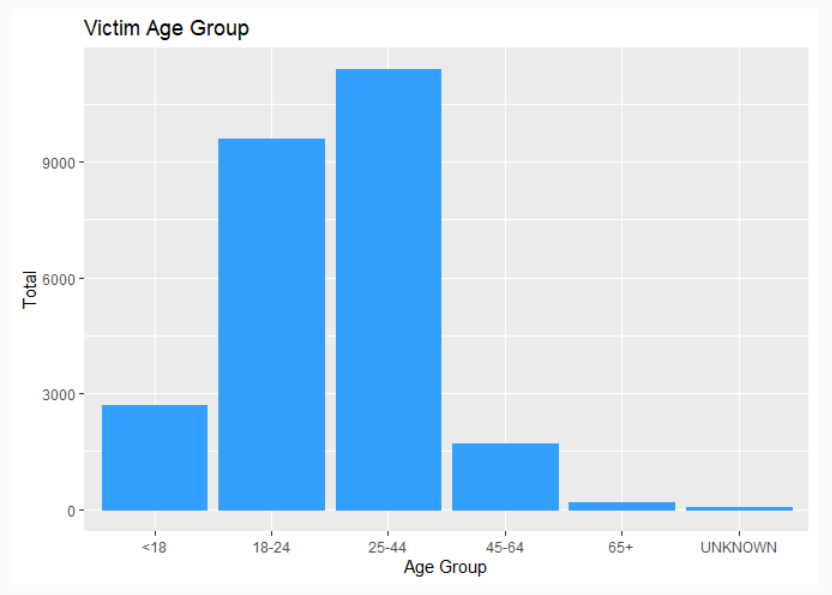
As in the case of perpetrators the majority of victims are male, there are much less female victims.
vic_sex_plot <- ggplot(data=shooting_data_vic_sex, aes(x=VIC_SEX, y=n)) +
  geom_bar(stat='identity', color = "#339FFF", fill = "#339FFF") +
  ggtitle("Victim Sex") + xlab("Sex") + ylab("Total")

vic_sex_plot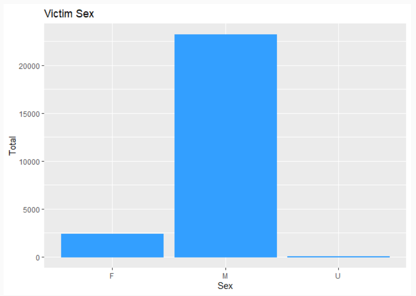
The last category of victims that I wanted to look at, was race. We can again see that most victims are black. However, without knowing the overall population distribution it is difficult to draw any conclusions. It might be possible that the majority of the population is black people.
vic_race_plot <- ggplot(data=shooting_data_vic_race, aes(x=reorder(VIC_RACE,(n)), y=n, color = VIC_RACE, fill = VIC_RACE)) +
  geom_bar(stat='identity') +
  theme(axis.text.x=element_blank(), axis.ticks.x=element_blank()) +
  ggtitle("Victim Race") + xlab("Race") + ylab("Total")

vic_race_plot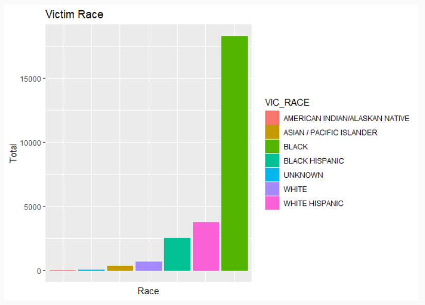
4 Bias Identification
Without extra data about the population distribution it is very easy to draw conclusions and introduce a bias towards a borough, a specific age group or a race. I am not familiar with the demographics of these areas and therefore, I must be extra careful of introducing a bias towards a specific area of the analysis.
5 Conclusion
From the analysis we can see that Brooklyn is the Borough with the most shootings, (10365 shootings or 40.5%) in total and Staten Island the least with 736 shootings or 2.9%. Out of a Total of 25,596 shootings between 2006 and 2021, 4928 people died (19.3%) and 20668 survived the shooting (80.7%). There are some missing values from the shooter’s information, and I assume that it is because they were not apprehended yet. It is interesting to see that the number of shooters between 18 and 24 as well as 25 and 44 are very close to each other. There are 5844 shooters between 18 and 24 (35.9%) and 5202 shooters between 25 and 44 (31.9%). The most victims are between 25 and 44, 11386 to be exact or (44.5%) and 9604 between 18 and 24 (37.5%). Most shootings happen between males, 14416 shooters (97.5%) and 23182 victims (90.6%). The last comparison between shooters and victims are based on race. It looks like black-on-black violence is a big problem with black shooters representing 10668 of the incidents (73.8%) and black victims representing 18281 of the incidents (71.4%). It might also be possible that black people represent a much larger proportion of the overall population. I do not have population data and could not investigate this further. The most shootings happened at night around midnight.