Analytics Queries on Real Car Wash Data
In Phase 4 the data finally talks back. With 2,613 rows loaded across five tables, we ran three analytical SQL queries that answer real business questions — member health, revenue trends, and location performance. Along the way we hit three of the most important SQL patterns in data engineering: window functions, CTEs, and period-over-period comparisons with LAG().
Where We Are in the Series
Phases 1–3 were all infrastructure: environment setup, table design, and data loading. Phase 4 is where we start getting answers. The data is real, the schema is clean, and Snowflake’s SQL engine is ready. Three queries, three insights, three SQL patterns worth knowing deeply.
🗂️ What You’ll Learn in This Post
How window functions work — and when to use SUM() OVER () vs GROUP BY. How LAG() calculates month-over-month growth in a single query. How CTEs make complex queries readable and reusable. The actual results from our car wash data — member health, MRR trend, and location rankings. Why COUNT(*) and COUNT(DISTINCT col) are completely different things.
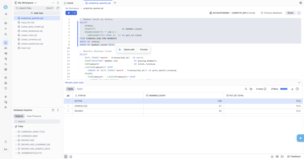
Query 1 — Member Count by Status
The simplest question in any membership business: how many members do we actually have, and what state are they in? This query answers it with percentages so the numbers have context even as the member base grows.
| STATUS | MEMBER_COUNT | PCT_OF_TOTAL | Business Interpretation |
|---|---|---|---|
| ACTIVE | 148 | 74.0% | Core revenue base — these members billed monthly |
| CANCELLED | 27 | 13.5% | Churned members — lost MRR, lifecycle state = ‘churned’ |
| PAUSED | 25 | 12.5% | At-risk — not cancelled yet but not paying either |
What the Results Actually Mean
74% active is a healthy baseline for a membership business — but the story is in the other 26%. PAUSED (12.5%) is the interesting segment: these members haven’t cancelled yet, which means they’re still reachable. In a real CRM workflow, a paused member would trigger a win-back campaign — a discount offer or a free month. This is exactly the kind of signal that feeds into Braze segments.
CANCELLED at 13.5% represents lost MRR. At $24.99 average plan price, 27 cancelled members is roughly $675/month in churned revenue. Small at this scale, but a number the business needs to track month over month.
The SQL Pattern — Window Function for Percentages
The clever part of this query is the percentage calculation. Most beginners would write two separate queries: one for count by status, one for total count, then divide manually. The window function does it in one:
SUM(COUNT(*)) OVER () is a window function applied on top of the GROUP BY result. The OVER () with empty parentheses means ‘across all rows in the result set’ — so while COUNT(*) gives the count per status group, SUM(COUNT(*)) OVER () gives the grand total across all groups. Dividing one by the other gives the percentage. No subquery. No CTE. One line.
💡 Window Functions vs GROUP BY — The Key Difference
GROUP BY collapses rows into one row per group and lets you aggregate within each group. Window functions compute aggregations across rows without collapsing them — each row keeps its own identity but gains access to a calculation that spans multiple rows. SUM() OVER () is the simplest window function: no partitioning, no ordering, just a grand total that every row in the result can see simultaneously.
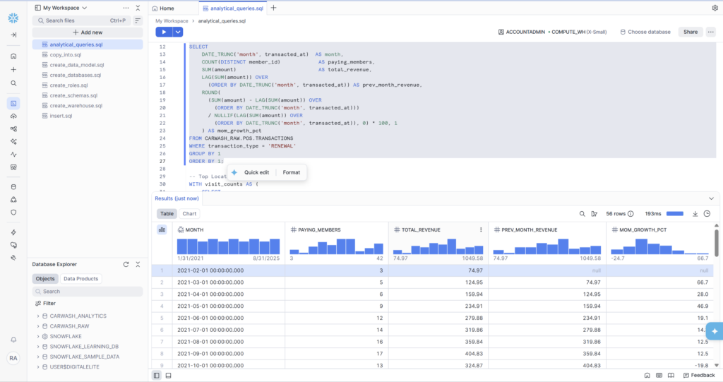
Query 2 — Monthly Revenue Trend with MoM Growth
This is the most technically rich query in Phase 4. It calculates monthly recurring revenue (MRR) for each month in the dataset, compares it to the previous month using LAG(), and computes the month-over-month growth percentage — all in a single SQL statement.
Breaking Down the Results
56 rows — one per month from February 2021 through September 2025. The first row correctly shows null for PREV_MONTH_REVENUE and MOM_GROWTH_PCT because there’s no prior month to compare to. Row 2 shows 66.7% growth — from $74.97 to $124.95 — because new members enrolled and started renewing in March.
The sparkline charts that Snowsight auto-generates above each numeric column are immediately useful: TOTAL_REVENUE shows a clear upward trend over 4+ years with seasonal dips, which is exactly what you’d expect from a growing multi-location subscription business.
Three SQL Patterns in This Query
1. DATE_TRUNC(‘month’, transacted_at) — truncates a timestamp to the first day of its month. 2024-03-15 09:32:00 becomes 2024-03-01 00:00:00. This is how you group timestamps into monthly buckets for trend analysis. Used in both the SELECT and the GROUP BY (which is why GROUP BY 1 works — it references the first column position).
2. LAG(col) OVER (ORDER BY …) — returns the value from the previous row in the specified order. When the data is ordered by month, LAG(SUM(amount)) gives you last month’s revenue on the current month’s row. This is the canonical pattern for any period-over-period comparison in SQL — MoM, QoQ, YoY all use the same structure.
3. NULLIF(expression, 0) — returns NULL instead of 0 when the expression equals zero. This prevents division-by-zero errors. Without it, the MoM calculation would fail in any month where previous revenue was exactly zero. NULLIF is a small detail that separates production-grade SQL from tutorial SQL.
📊 The WHERE transaction_type = ‘RENEWAL’ Filter
Notice the query filters to RENEWAL transactions only. This is intentional. MRR (Monthly Recurring Revenue) specifically measures predictable, repeating revenue. SIGNUP transactions are one-time events. UPGRADE transactions are anomalies. CHARGEBACK transactions are negative. Including all four would inflate or distort the revenue trend and make it useless for forecasting. Filtering to RENEWAL gives you a clean MRR signal.
Query 3 — Top Locations by Visit Volume
The third query ranks all 8 locations by total visit count and unique members. It uses a CTE (Common Table Expression) to keep the logic readable, and introduces the RANK() window function to assign a position to each location.
| RANK | LOCATION | STATE | TOTAL_VISITS | UNIQUE_MEMBERS |
|---|---|---|---|---|
| 1 | Indianapolis South | IN | 228 | 91 |
| 2 | Chicago Loop | IL | 212 | 81 |
| 3 | Columbus East | OH | 206 | 77 |
| 4 | Minneapolis West | MN | 178 | 69 |
| 5 | Indianapolis North | IN | 162 | 70 |
| 6 | Cincinnati West | OH | 114 | 82 |
| 7 | Milwaukee North | WI | 102 | 79 |
| 8 | St. Louis Central | MO | 91 | 70 |
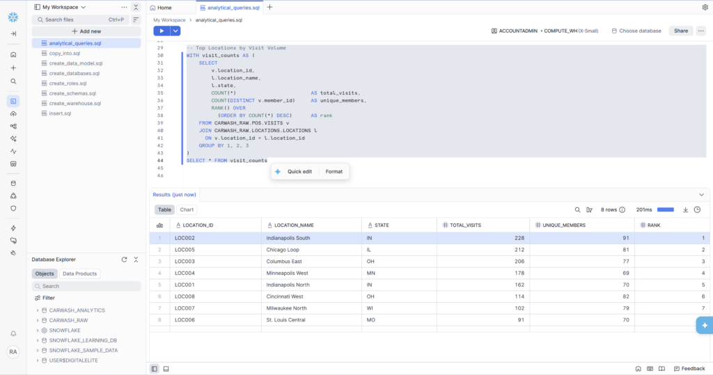
Indianapolis South leads with 228 visits and 91 unique members — the highest visit density in the network. Chicago Loop is second with 212 visits despite only 81 unique members, meaning Chicago customers visit more frequently per member. That’s a signal worth investigating: are Chicago members on higher-tier plans? Do they live closer to the location?
St. Louis Central sits at the bottom with 91 visits. It also opened most recently (January 2023 in our dataset), so lower volume is expected — but the RANK() makes the underperformance visible and gives operations something to act on.
The SQL Pattern — CTEs for Readable Logic
WITH visit_counts AS (…) is a CTE — a named subquery that can be referenced like a table. It doesn’t change what the query does. It changes how readable it is. The alternative — nesting the entire subquery inside the outer SELECT — produces the same result but becomes nearly impossible to debug or modify. CTEs are how you structure complex SQL so a colleague (or future you) can understand it six months later.
COUNT(*) vs COUNT(DISTINCT member_id)
This query uses both in the same SELECT — and they measure different things:
- COUNT(*) counts every row — so if member X visited location Y five times, they contribute 5 to total_visits
- COUNT(DISTINCT member_id) counts unique members — the same member X contributes 1 to unique_members regardless of how many times they visited
Both numbers are useful. TOTAL_VISITS tells you how busy a location is. UNIQUE_MEMBERS tells you how wide its reach is. A location with high visits but low unique members has a loyal core — good for retention but potentially limited in growth. A location with high unique members but lower visit frequency might need engagement campaigns to drive repeat visits.
Window Functions — The Pattern That Runs Through All Three Queries
Every query in Phase 4 uses at least one window function. This is not accidental — window functions are the single most important SQL concept for analytics engineering. Here’s the complete set used in this phase:
| Function | What It Does | Used In This Phase |
|---|---|---|
| SUM() OVER () | $Grand total across all rows for percentage calc | PCT_OF_TOTAL in member status query |
| LAG(col) OVER (ORDER BY …) | Previous row’s value in an ordered sequence | PREV_MONTH_REVENUE in revenue trend |
| RANK() OVER (ORDER BY … DESC) | Assigns rank 1, 2, 3… based on sort order | Location ranking by visit volume |
| COUNT(DISTINCT col) | Unique count — not the same as COUNT(*) | UNIQUE_MEMBERS per location |
Phase 4 Complete — What We Learned From the Data
✅ Phase 4 Deliverables — All Complete
- Query 1: Member status breakdown — 148 ACTIVE (74%), 27 CANCELLED (13.5%), 25 PAUSED (12.5%)
- Query 2: 56 months of MRR trend data — Feb 2021 through Sep 2025, with MoM growth %
- Query 3: All 8 locations ranked — Indianapolis South #1 (228 visits), St. Louis Central #8 (91 visits)
- SQL patterns covered: SUM() OVER (), LAG() OVER (ORDER BY), RANK() OVER (ORDER BY), DATE_TRUNC(), NULLIF(), CTEs
- Business insights: 26% of members need CRM attention (PAUSED + CANCELLED segments)
- All queries saved in analytical_queries.sql in Snowsight workspace